复习下 Logistic 回归基础
文章目录
整体参考了 Manny Gimond 的 一篇博文:Logistic regression。
数据使用的是 mlbench 包里的 PimaIndiansDiabetes2。这是一个根据患者年龄、BMI、怀孕次数、OGTT 后胰岛素水平和 OGTT(口服糖耐量试验)血糖结果等等变量预测糖尿病(二分类,Neg vs. Pos)的数据,正好可以作为 Logistic 回归的例子。具体介绍可以参看 Kaggle Pima Indians Diabetes Database: Predict the onset of diabetes based on diagnostic measures
用到的包不多,主要就是数据清洗和可视化,rms 希望有机会(又挖坑了嘿)可以深入学习一下,这里只是简单用一下。
library("dplyr")
library("ggplot2")
library("ggbeeswarm")
library("beeswarm")
library("rms")
library("pscl") # McFadden R2

set.seed(1234)

theme_set(theme_minimal())
数据
载入数据之后发现数据里有缺失值,这里图方便直接就不要含缺失值的数据了。然后把 BMI 从连续型变量切分成因子类,由于低体重组人数太少(只有一个)直接合并到正常体重组了。
data("PimaIndiansDiabetes2", package="mlbench")
head(PimaIndiansDiabetes2)
##   pregnant glucose pressure triceps insulin mass pedigree age diabetes
## 1        6     148       72      35      NA 33.6    0.627  50      pos
## 2        1      85       66      29      NA 26.6    0.351  31      neg
## 3        8     183       64      NA      NA 23.3    0.672  32      pos
## 4        1      89       66      23      94 28.1    0.167  21      neg
## 5        0     137       40      35     168 43.1    2.288  33      pos
## 6        5     116       74      NA      NA 25.6    0.201  30      neg

dim(PimaIndiansDiabetes2)
## [1] 768   9


sapply(PimaIndiansDiabetes2, function(x) sum(is.na(x)))
## pregnant  glucose pressure  triceps  insulin     mass pedigree      age
##        0        5       35      227      374       11        0        0
## diabetes
##        0

dbt <- tibble(PimaIndiansDiabetes2) %>%
  na.omit() %>%
  mutate(bmi = factor(case_when(
    # mass < 18.5 ~ "underweight",
    mass < 25 ~ "normal",
    mass >= 25 & mass < 30 ~ "overweight",
    mass >= 30 ~ "obese"),
    levels = c("normal", "overweight", "obese"))
    ) %>%
  select(-mass)
levels(dbt$diabetes) <- c(0, 1)

# rms option
dd <- datadist(dbt)
options(datadist = "dd")
先来看看很明显的,糖尿病和非糖尿病两组之间血糖是一样的吗?假装并不知道血糖高说明有糖尿病….
par(mar = c(4.1, 4.1, 1.1, 2.1))
boxplot(glucose ~ diabetes, data = dbt,
        col = "white",
        outline = FALSE)
beeswarm(glucose ~ diabetes, data = dbt,
         pch = 21, col = 2:3,
         bg = "grey",
         add = TRUE)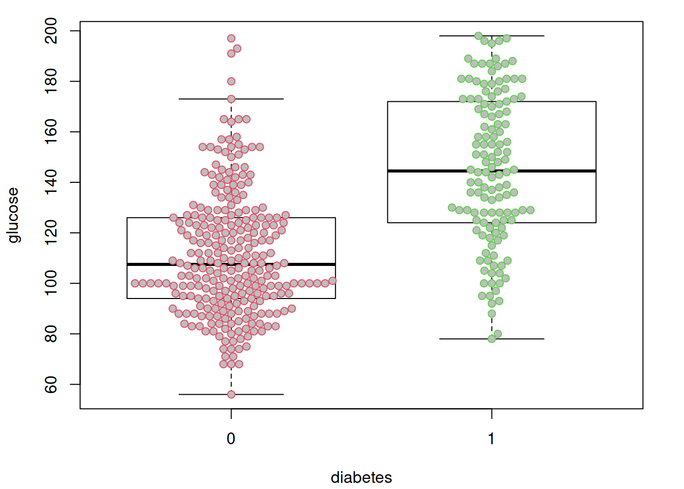
p1 <- grDevices::recordPlot()这里插播两个小东西: ggplot 版的的 beeswarm 图,由 ggbeeswarm 提供;以及grDevices::recordPlot() 这个黑魔法。两个图放在一起对比一下():
p2 <- ggplot(dbt, aes(x= diabetes, y = glucose)) +
    geom_boxplot(width = 1/2, outlier.shape = NA) +
    geom_beeswarm(alpha = 1/3) +
    labs(x = "Diabetes",
         y = "OGTT Plasma glucose conc.") +
    NULL

cowplot::plot_grid(p1, p2,
                   # rel_widths = c(1, 2),
                   ncol = 2)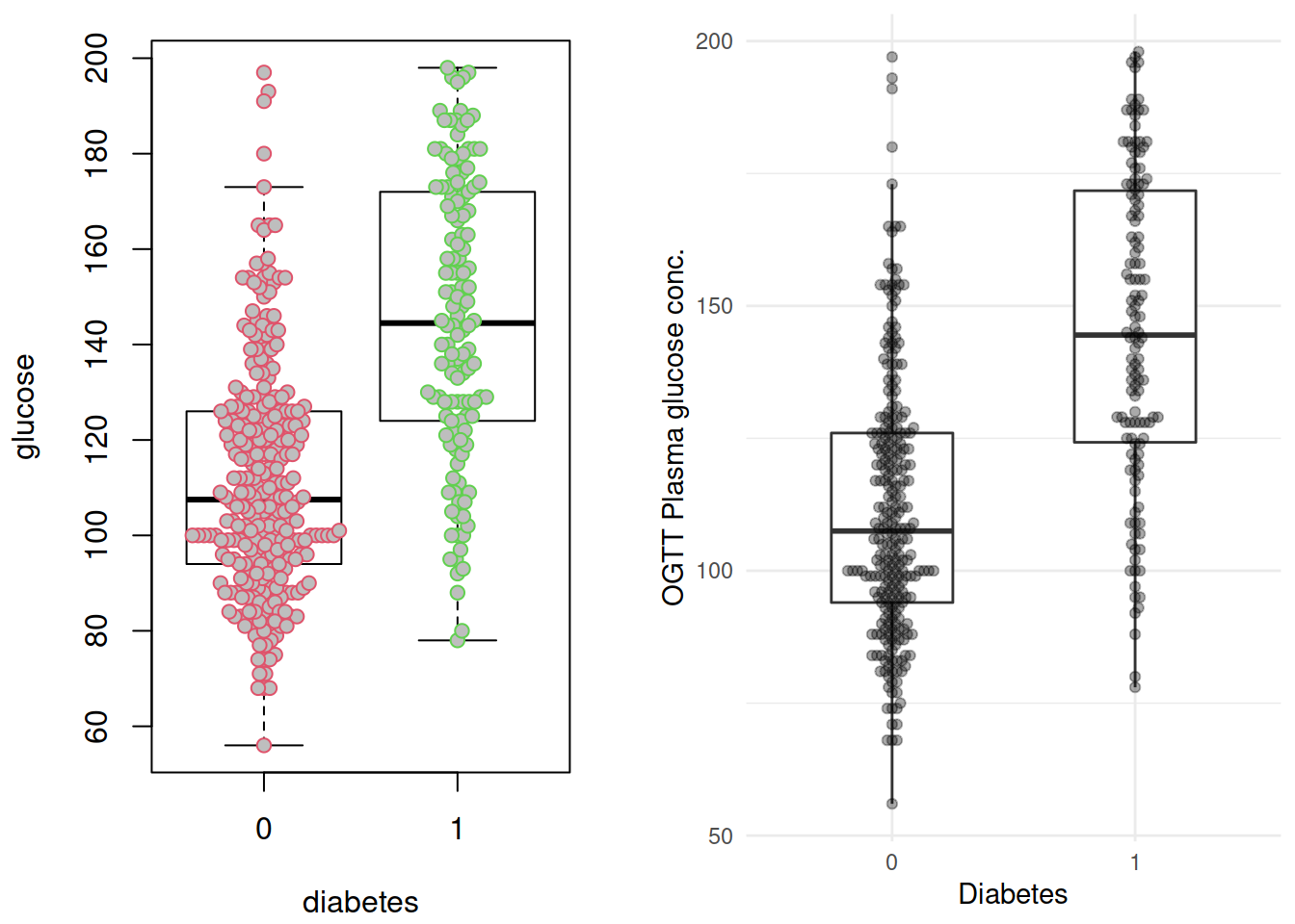
不出所料,糖尿病患者血糖水平似乎更高。
再来把坐标轴转换一下,如果血糖水平作为横轴、糖尿病是否作为纵轴会是什么样子?
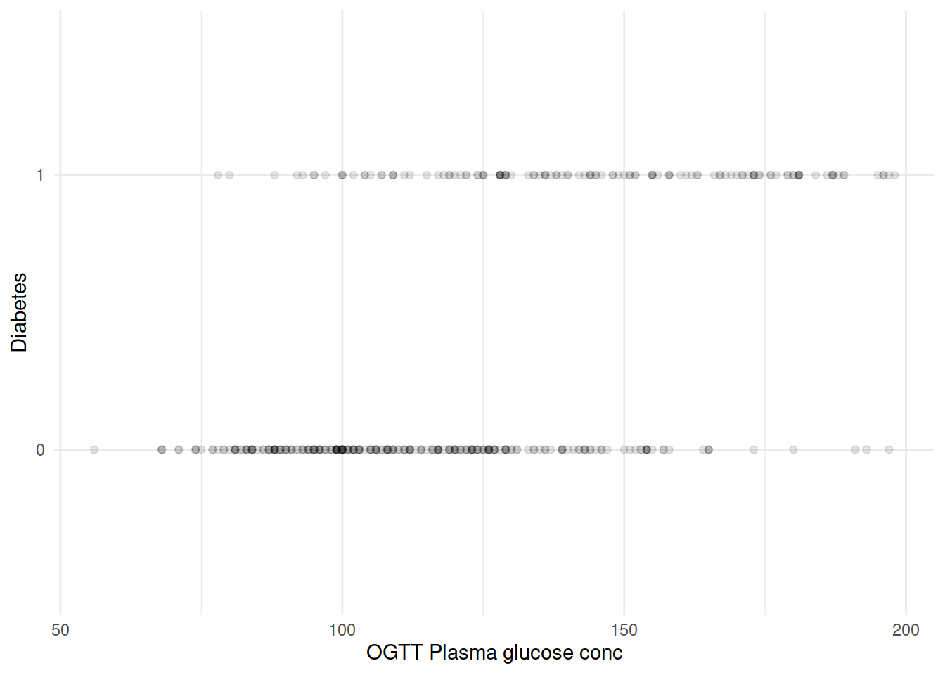
由于 diabetes 只取 0/1,大量散点相互覆盖。
尝试用不同的方法取拟合一条曲线来看变量之间的关系:
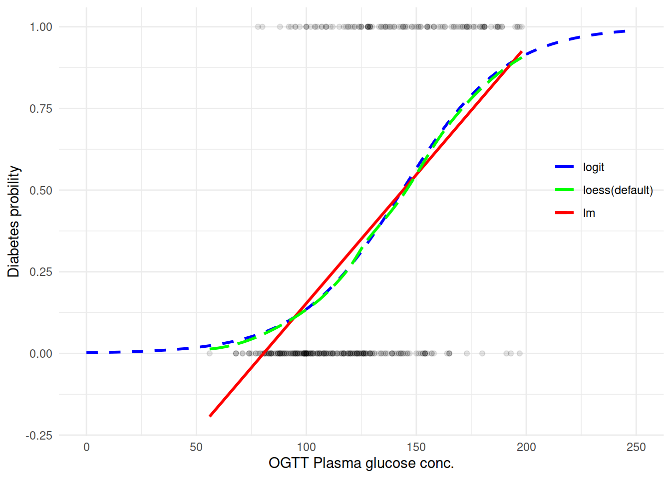
能看到确实 logit 拟合还是不错的样子。直接来上 Logistic 回归模型吧:
模型 1
M1 <- glm(diabetes ~ glucose, family = binomial, data = dbt)
M1
##
## Call:  glm(formula = diabetes ~ glucose, family = binomial, data = dbt)
##
## Coefficients:
## (Intercept)      glucose
##    -6.09552      0.04242
##
## Degrees of Freedom: 391 Total (i.e. Null);  390 Residual
## Null Deviance:       498.1
## Residual Deviance: 386.7     AIC: 390.7

summary(M1)
##
## Call:
## glm(formula = diabetes ~ glucose, family = binomial, data = dbt)
##
## Deviance Residuals:
##     Min       1Q   Median       3Q      Max
## -2.1728  -0.7475  -0.4789   0.7153   2.3860
##
## Coefficients:
##              Estimate Std. Error z value Pr(>|z|)
## (Intercept) -6.095521   0.629787  -9.679   <2e-16 ***
## glucose      0.042421   0.004761   8.911   <2e-16 ***
## ---
## Signif. codes:  0 '***' 0.001 '**' 0.01 '*' 0.05 '.' 0.1 ' ' 1
##
## (Dispersion parameter for binomial family taken to be 1)
##
##     Null deviance: 498.10  on 391  degrees of freedom
## Residual deviance: 386.67  on 390  degrees of freedom
## AIC: 390.67
##
## Number of Fisher Scoring iterations: 4

round(exp(cbind(OR = coef(M1), confint(M1))), 2)
## Waiting for profiling to be done...
##               OR 2.5 % 97.5 %
## (Intercept) 0.00  0.00   0.01
## glucose     1.04  1.03   1.05
首先 glucose 显著相关(of course),系数是 0.04 表明是血糖高糖尿病可能性也提高(不一定是因果,只说明正相关)。 模型 AIC 370.9,残差 386.7,Null 模型(只有截距)的残差 498.1。可以看到即使加入一个显著解释变量的时候残差也“明显”降低了(“明显”打了引号是因为这只是直觉上的明显降低,至于是否真的降低要用统计检验来证明。后面模型诊断评价涉及)。
用这个模型来预测糖尿病看看之前的曲线会是什么样子:
M.df <- data.frame(glucose = seq(0, 300, 1))
M.df$diabetes = predict(M1, newdata = M.df, type = "response")
生成新的预测数据之后,再来用这个数据作图:
ggplot(M.df, aes(x = glucose, y = diabetes)) +
  geom_line(size = 1.2, aes(color = "blue"), alpha = 1/2) +
  geom_point(data = dbt,
             aes(glucose, as.numeric(diabetes) - 1),
             alpha = 1/10) +
  geom_smooth(data = dbt, formula = y ~ x,
              method = "glm", method.args = list(family = "binomial"),
              se = FALSE,
              size = .5,
             aes(glucose, as.numeric(diabetes) - 1, color = "red")) +
  scale_color_manual(name = "",
                       values = c("blue" = "blue",
                                  "red" = "red"),
                       labels = c("Predicted data", "Real data")) +
  labs(y = "Diabetes probility",
       x = "OGTT Plasma glucose conc.") +
  theme(legend.position = c(.9, .5)) +
  NULL
模型评价
在线性模型里,一个很重要的评价模型的参数就是 \(R^2\),它表示模型可解释的变异占总变异的比例。很显然,这个比例越高越好。
Logistic 回归是一种广义线性模型。如果还用 \(R^2\) 来评价模型,就得到所谓“伪” R 方,pseudo \(R^2\),也叫 McFadden’s \(R^2\) 。可以根据它的定义自己计算,也可以直接用 pscl 包的 pR2():
-2 * logLik(M1)
## 'log Lik.' 386.666 (df=2)
M1$deviance
## [1] 386.666

-2 * logLik(update(M1, .~. - glucose))
## 'log Lik.' 498.0978 (df=1)
M1$null.deviance
## [1] 498.0978


M1.pseudo.R2 <- (M1$null.deviance - M1$deviance) / M1$null.deviance
M1.pseudo.R2
## [1] 0.2237148

pR2(M1)["McFadden"]
## fitting null model for pseudo-r2
##  McFadden
## 0.2237148
参考 StackExchange: McFadden’s Pseudo-\(R^2\) Interpretation,0.2 - 0.4 之间认为模型表现 OK (excellent performance)。
另外对于模型评价还有其他一些指标,在 rms 包 lrm() 可以非常方便的得到:
M1.lrm <- lrm(diabetes ~ glucose, data = dbt)
M1.lrm
## Logistic Regression Model
##
##  lrm(formula = diabetes ~ glucose, data = dbt)
##
##                         Model Likelihood    Discrimination    Rank Discrim.
##                               Ratio Test           Indexes          Indexes
##  Obs           392    LR chi2     111.43    R2       0.344    C       0.806
##   0            262    d.f.             1    g        1.481    Dxy     0.612
##   1            130    Pr(> chi2) <0.0001    gr       4.398    gamma   0.616
##  max |deriv| 3e-12                          gp       0.271    tau-a   0.272
##                                             Brier    0.161
##
##            Coef    S.E.   Wald Z Pr(>|Z|)
##  Intercept -6.0955 0.6298 -9.68  <0.0001
##  glucose    0.0424 0.0048  8.91  <0.0001
##

summary(M1.lrm)
##              Effects              Response : diabetes
##
##  Factor      Low High Diff. Effect S.E.    Lower 0.95 Upper 0.95
##  glucose     99  143  44    1.8665 0.20947 1.4560     2.2771
##   Odds Ratio 99  143  44    6.4658      NA 4.2886     9.7481

M1.lrm$stats[c("R2", "Brier", "C", "Dxy")]
##        R2     Brier         C       Dxy
## 0.3439656 0.1610583 0.8057692 0.6115385
这里给出的信息很丰富,捡几个常见的说一下:
- R2 是 the Nagelkerke R^2 index,具体计算公式不列了,取值范围 0~1。是 Discrimination 参数
- Brier score 在文献里也经常看到,计算方法就是预测值和观察值差值的平方和除以观测数。
DescTools::BrierScore()也可以计算,或者依据公式其实就是mean((M1$y - M1$fitted.values)^2)的结果 越小表示模型预测约准确。Discrimination 参数 - C 就是经常见到的 C 统计量,C statistic,Concordance index,和 AUC 是相等的
- Dxy 是 Somers’ D, 具体公式不给了,略复杂。对于 Logistic 回归,Dxy = 2 * (AUC - 0.5)
- Dxy 和 Tau-a 的具体介绍可以看 Logistic regression, Gamma (Goodman and Kruskal Gamma),文末把这篇博文的代码附上
比较不同模型之间是否有统计学差异,用卡方检验,卡方值是两模型残差相减,自由度两模型自由度之差。比如前面提到 M1 只是有一个变量 glucose 的时候模型残差已经明显降低,那相比 Null 模型,M1 是不是真的“统计学显著地显著”更好呢?
(M1Chidf <- M1$df.null - M1$df.residual)
## [1] 1
(M1Chi <- M1$null.deviance - M1$deviance)
## [1] 111.4318
(M1chisq.prob <- 1 - pchisq(M1Chi, M1Chidf))
## [1] 0

# 或者一步计算
with(M1, pchisq(null.deviance - deviance,
                df.null - df.residual,
                lower.tail = FALSE))
## [1] 4.758898e-26
对照输出参看 M1.lrm 可以看到 Model Likelihood 那里的输出就是这里的计算结果。
现在在 M1 的基础上再添加一个变量 bmi:
M2 <- glm(diabetes ~ glucose + bmi, dbt, family = binomial)
summary(M2)
##
## Call:
## glm(formula = diabetes ~ glucose + bmi, family = binomial, data = dbt)
##
## Deviance Residuals:
##     Min       1Q   Median       3Q      Max
## -2.2285  -0.7236  -0.4207   0.6675   2.6183
##
## Coefficients:
##                Estimate Std. Error z value Pr(>|z|)
## (Intercept)   -7.665634   0.954940  -8.027 9.96e-16 ***
## glucose        0.039914   0.004854   8.223  < 2e-16 ***
## bmioverweight  1.386848   0.798458   1.737  0.08240 .
## bmiobese       2.198471   0.756548   2.906  0.00366 **
## ---
## Signif. codes:  0 '***' 0.001 '**' 0.01 '*' 0.05 '.' 0.1 ' ' 1
##
## (Dispersion parameter for binomial family taken to be 1)
##
##     Null deviance: 498.1  on 391  degrees of freedom
## Residual deviance: 368.4  on 388  degrees of freedom
## AIC: 376.4
##
## Number of Fisher Scoring iterations: 5

round(exp(cbind(OR = coef(M2), confint(M2))), 2)
## Waiting for profiling to be done...
##                 OR 2.5 % 97.5 %
## (Intercept)   0.00  0.00   0.00
## glucose       1.04  1.03   1.05
## bmioverweight 4.00  1.01  26.94
## bmiobese      9.01  2.54  57.61

M2.pseudo.R2 <- (M2$null.deviance - M2$deviance) / M2$null.deviance
M2.pseudo.R2
## [1] 0.2603819


with(M2, pchisq(null.deviance - deviance,
                df.null - df.residual,
                lower.tail = FALSE))
## [1] 6.290107e-28

M2.lrm <- lrm(diabetes ~ glucose + bmi, data = dbt)
M2.lrm
## Logistic Regression Model
##
##  lrm(formula = diabetes ~ glucose + bmi, data = dbt)
##
##                          Model Likelihood    Discrimination    Rank Discrim.
##                                Ratio Test           Indexes          Indexes
##  Obs            392    LR chi2     129.70    R2       0.392    C       0.830
##   0             262    d.f.             3    g        1.772    Dxy     0.660
##   1             130    Pr(> chi2) <0.0001    gr       5.883    gamma   0.663
##  max |deriv| 0.0008                          gp       0.291    tau-a   0.293
##                                              Brier    0.154
##
##                 Coef    S.E.   Wald Z Pr(>|Z|)
##  Intercept      -7.6656 0.9552 -8.02  <0.0001
##  glucose         0.0399 0.0049  8.22  <0.0001
##  bmi=overweight  1.3868 0.7988  1.74  0.0825
##  bmi=obese       2.1985 0.7569  2.90  0.0037
##

summary(M2.lrm)
##              Effects              Response : diabetes
##
##  Factor                 Low High Diff. Effect   S.E.    Lower 0.95 Upper 0.95
##  glucose                99  143  44     1.75620 0.21356  1.337600   2.17480
##   Odds Ratio            99  143  44     5.79040      NA  3.810000   8.80030
##  bmi - normal:obese      3    1  NA    -2.19850 0.75688 -3.681900  -0.71500
##   Odds Ratio             3    1  NA     0.11097      NA  0.025174   0.48919
##  bmi - overweight:obese  3    2  NA    -0.81162 0.32839 -1.455200  -0.16800
##   Odds Ratio             3    2  NA     0.44414      NA  0.233340   0.84535
M2 在 M1 的基础上多个模型参数都有提升,一样的,统计学显著吗?
anova(M1, M2, test = "Chi")
## Analysis of Deviance Table
##
## Model 1: diabetes ~ glucose
## Model 2: diabetes ~ glucose + bmi
##   Resid. Df Resid. Dev Df Deviance  Pr(>Chi)
## 1       390     386.67
## 2       388     368.40  2   18.264 0.0001082 ***
## ---
## Signif. codes:  0 '***' 0.001 '**' 0.01 '*' 0.05 '.' 0.1 ' ' 1


lrtest(M1.lrm, M2.lrm)
##
## Model 1: diabetes ~ glucose
## Model 2: diabetes ~ glucose + bmi
##
##   L.R. Chisq         d.f.            P
## 1.826383e+01 2.000000e+00 1.081583e-04
卡方检验显示 M2 明显优于 M1。
下面涉及到模型的校准(calibration),rms 做起来很方便,就直接用 rms 来继续吧:
简单看看 rms
首先是通过 bootstrap 内部验证(internal-validation)来看模型是否有明显过拟合:
M1.lrm <- lrm(diabetes ~ glucose, data = dbt,
              x = TRUE, y = TRUE)
M1.lrm
## Logistic Regression Model
##
##  lrm(formula = diabetes ~ glucose, data = dbt, x = TRUE, y = TRUE)
##
##                         Model Likelihood    Discrimination    Rank Discrim.
##                               Ratio Test           Indexes          Indexes
##  Obs           392    LR chi2     111.43    R2       0.344    C       0.806
##   0            262    d.f.             1    g        1.481    Dxy     0.612
##   1            130    Pr(> chi2) <0.0001    gr       4.398    gamma   0.616
##  max |deriv| 3e-12                          gp       0.271    tau-a   0.272
##                                             Brier    0.161
##
##            Coef    S.E.   Wald Z Pr(>|Z|)
##  Intercept -6.0955 0.6298 -9.68  <0.0001
##  glucose    0.0424 0.0048  8.91  <0.0001
##


M1.valid <- validate(M1.lrm, method = "boot", B = 1000)
M1.valid
##           index.orig training   test optimism index.corrected    n
## Dxy           0.6115   0.6116 0.6115   0.0001          0.6115 1000
## R2            0.3440   0.3454 0.3440   0.0015          0.3425 1000
## Intercept     0.0000   0.0000 0.0055  -0.0055          0.0055 1000
## Slope         1.0000   1.0000 1.0023  -0.0023          1.0023 1000
## Emax          0.0000   0.0000 0.0016   0.0016          0.0016 1000
## D             0.2817   0.2840 0.2817   0.0023          0.2794 1000
## U            -0.0051  -0.0051 0.0003  -0.0054          0.0003 1000
## Q             0.2868   0.2891 0.2814   0.0077          0.2791 1000
## B             0.1611   0.1603 0.1619  -0.0017          0.1627 1000
## g             1.4812   1.4920 1.4812   0.0109          1.4703 1000
## gp            0.2709   0.2701 0.2709  -0.0008          0.2717 1000


M2.lrm <- lrm(diabetes ~ glucose + bmi, data = dbt,
              x = TRUE, y = TRUE)
M2.lrm
## Logistic Regression Model
##
##  lrm(formula = diabetes ~ glucose + bmi, data = dbt, x = TRUE,
##      y = TRUE)
##
##                          Model Likelihood    Discrimination    Rank Discrim.
##                                Ratio Test           Indexes          Indexes
##  Obs            392    LR chi2     129.70    R2       0.392    C       0.830
##   0             262    d.f.             3    g        1.772    Dxy     0.660
##   1             130    Pr(> chi2) <0.0001    gr       5.883    gamma   0.663
##  max |deriv| 0.0008                          gp       0.291    tau-a   0.293
##                                              Brier    0.154
##
##                 Coef    S.E.   Wald Z Pr(>|Z|)
##  Intercept      -7.6656 0.9552 -8.02  <0.0001
##  glucose         0.0399 0.0049  8.22  <0.0001
##  bmi=overweight  1.3868 0.7988  1.74  0.0825
##  bmi=obese       2.1985 0.7569  2.90  0.0037
##


M2.valid <- validate(M2.lrm, method = "boot", B = 1000)
M2.valid
##           index.orig training    test optimism index.corrected    n
## Dxy           0.6603   0.6628  0.6557   0.0071          0.6532 1000
## R2            0.3916   0.3982  0.3807   0.0176          0.3740 1000
## Intercept     0.0000   0.0000 -0.0234   0.0234         -0.0234 1000
## Slope         1.0000   1.0000  0.9603   0.0397          0.9603 1000
## Emax          0.0000   0.0000  0.0129   0.0129          0.0129 1000
## D             0.3283   0.3361  0.3176   0.0185          0.3098 1000
## U            -0.0051  -0.0051  0.0019  -0.0070          0.0019 1000
## Q             0.3334   0.3412  0.3157   0.0255          0.3079 1000
## B             0.1540   0.1526  0.1556  -0.0030          0.1570 1000
## g             1.7720   1.9877  1.8597   0.1280          1.6441 1000
## gp            0.2910   0.2920  0.2859   0.0061          0.2849 1000
给出的结果里 Dxy 和 R^2 分别有 training 和 test 的值已经据此计算出的 optimism,然后给出了校正值。这里可以看到其实 M1、M2 的过拟合不明显。
做 Calibration 曲线图:
myPlotCalib <- function (x, xlab, ylab, xlim, ylim,
                         legend = TRUE, subtitles = TRUE,
                        cols = c("red", "darkgreen", "black"),
                        lty = c(2, 3, 1),
                        cex.subtitles = 0.75, riskdist = TRUE,
                        scat1d.opts = list(nhistSpike = 200), ...)
{
    at <- attributes(x)
    if (missing(ylab))
        ylab <- if (at$model == "lr")
            "Actual Probability"
    else paste("Observed", at$yvar.name)
    if (missing(xlab)) {
        if (at$model == "lr") {
            xlab <- paste("Predicted Pr{", at$yvar.name, sep = "")
            if (at$non.slopes == 1) {
                xlab <- if (at$lev.name == "TRUE")
                    paste(xlab, "}", sep = "")
                else paste(xlab, "=", at$lev.name, "}", sep = "")
            }
            else xlab <- paste(xlab, ">=", at$lev.name, "}",
                               sep = "")
        }
        else xlab <- paste("Predicted", at$yvar.name)
    }
    p <- x[, "predy"]
    p.app <- x[, "calibrated.orig"]
    p.cal <- x[, "calibrated.corrected"]
    if (missing(xlim) & missing(ylim))
        xlim <- ylim <- range(c(p, p.app, p.cal), na.rm = TRUE)
    else {
        if (missing(xlim))
            xlim <- range(p)
        if (missing(ylim))
            ylim <- range(c(p.app, p.cal, na.rm = TRUE))
    }
    plot(p, p.app, xlim = xlim, ylim = ylim, xlab = xlab, ylab = ylab,
         type = "n", ...)
    predicted <- at$predicted
    err <- NULL
    if (length(predicted)) {
        s <- !is.na(p + p.cal)
        err <- predicted - approx(p[s], p.cal[s], xout = predicted,
                                  ties = mean)$y
        cat("\nn=", n <- length(err), "   Mean absolute error=",
            round(mae <- mean(abs(err), na.rm = TRUE), 3),
            "   Mean squared error=",
            round(mean(err^2, na.rm = TRUE), 5),
            "\n0.9 Quantile of absolute error=",
            round(quantile(abs(err), 0.9, na.rm = TRUE), 3),
            "\n\n", sep = "")
        if (subtitles)
            title(sub = paste("Mean absolute error=",
                              round(mae, 3), " n=", n, sep = ""),
                  cex.sub = cex.subtitles,
                  adj = 1)
        if (riskdist)
            do.call("scat1d", c(list(x = predicted), scat1d.opts))
    }
    lines(p, p.app, lty = lty[1], col = cols[1], lwd = 2)
    lines(p, p.cal, lty = lty[2], col = cols[2], lwd = 2)
    abline(a = 0, b = 1, lty = lty[3], col = cols[3])
    if (subtitles)
        title(sub = paste("B =", at$B, "repetitions,", at$method),
              cex.sub = cex.subtitles, adj = 0)
    if (!(is.logical(legend) && !legend)) {
        if (is.logical(legend))
            legend <- list(x = xlim[1] + 0.5 * diff(xlim), y = ylim[1] +
                               0.32 * diff(ylim))
        legend(legend, c("Apparent", "Bias-corrected", "Ideal"),
               lwd = 1.75, seg.len = 1, cex = .75,
               lty = lty, bty = "n", col = cols)
    }
    invisible(err)
}

par(mar = c(5.1, 4.1, 2, 0.5),
    mfrow = c(1, 2))
M1.calib <- calibrate(M1.lrm, method = "boot", B = 1000)
M2.calib <- calibrate(M2.lrm, method = "boot", B = 1000)

myPlotCalib(M1.calib, las = 1, main = "M1 Calibration", cex.subtitles = 0.5,
     xlab = "Predicted probability",
     ylab = "Observed probability")
##
## n=392   Mean absolute error=0.005   Mean squared error=5e-05
## 0.9 Quantile of absolute error=0.011
par(mar = c(5.1, 2.5, 2, 2.1))
myPlotCalib(M2.calib, las = 1,  main = "M2 Calibration", cex.subtitles = 0.5,
            xlab = "Predicted probability"
            )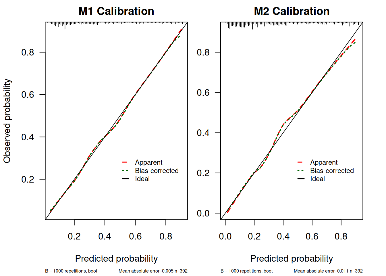
##
## n=392   Mean absolute error=0.011   Mean squared error=0.00026
## 0.9 Quantile of absolute error=0.03
这里由于嫌原来 rms 提供的作图函数不能自定义颜色所以自己把提取出来的函数改了一下(参考了 StackOverflow: Changing the colour of a calibration plot)。
这个图解释一下:
- 上面 X 轴的 rug plot 表示预测值的分布情况,可以看到多数病例 diabetes = 0, 当然可以自己
table(dbt$diabetes)验证一下 - 标记为“Apparent”的这条曲线就是样本内校准情况
- 标记为“Ideal”的是完美模型的情况,因为 x = y 即所有预测值和实际值完全相同
- 标记为“Bias Corrected” 的是通过 bootstrap 抽样校准了过拟合情况的结果,这也是理论上模型用到新数据中做预测时表现的预测情形。这条曲线也是考察模型外推性的依据
- Mean absolute error (MAE)是预测值和实际值平均绝对值差值了, Mean squared error(MSE) 就是均方差了,类比一下方差和标准差很好理解。
从这些结果看 M1.lrm 和 M2.lrm 的模型校准度也还可以,在 0.4 左右有一点点高估和低估。
附
在一篇博文里看到的计算 Dxy 和 Tau-a 的实现,没有深究,代码看一下:
# http://shashiasrblog.blogspot.com/2014/01/binary-logistic-regression-on-r.html
# Logistic regression, Gamma (Goodman and Kruskal Gamma),
# Somers' D, Kendall's Tau A

OptimisedConc = function(model)
{
  Data = cbind(model$y, model$fitted.values)
  ones = Data[Data[, 1] == 1, ]
  zeros = Data[Data[, 1] == 0, ]
  conc = matrix(0, dim(zeros)[1], dim(ones)[1])
  disc = matrix(0, dim(zeros)[1], dim(ones)[1])
  ties = matrix(0, dim(zeros)[1], dim(ones)[1])
  for (j in 1:dim(zeros)[1]) {
    for (i in 1:dim(ones)[1]) {
      if (ones[i, 2] > zeros[j, 2]) {
        conc[j, i] = 1
        }
      else if (ones[i, 2] < zeros[j, 2]) {
        disc[j, i] = 1
      }
      else if (ones[i, 2] == zeros[j, 2]) {
        ties[j, i] = 1
      }
    }
  }
  Pairs = dim(zeros)[1] * dim(ones)[1]
  PercentConcordance = (sum(conc) / Pairs) * 100
  PercentDiscordance = (sum(disc) / Pairs) * 100
  PercentTied = (sum(ties) / Pairs) * 100

  PercentConcordance = (sum(conc) / Pairs) * 100
  PercentDiscordance = (sum(disc) / Pairs) * 100
  PercentTied = (sum(ties) / Pairs) * 100
  N <- length(model$y)
  gamma <- (sum(conc) - sum(disc)) / Pairs
  Somers_D <- (sum(conc) - sum(disc)) / (Pairs - sum(ties))
  k_tau_a <- 2 * (sum(conc) - sum(disc)) / (N * (N - 1))
  return(list("Percent Concordance" = PercentConcordance,
      "Percent Discordance" = PercentDiscordance,
      "Percent Tied" = PercentTied,
      "Pairs" = Pairs,
      "Gamma" = gamma,
      "Somers D" = Somers_D,
      "Kendall's Tau A" = k_tau_a))

  # return(list("Percent Concordance" = PercentConcordance,
  # "Percent Discordance"=PercentDiscordance,
  # "Percent Tied" = PercentTied,
  # "Pairs" = Pairs))
}
还有一个实现多种拟合优度检验的实现:
#####################################################################
# NAME: Tom Loughin                                                 #
# DATE: 1-10-13                                                     #
# PURPOSE: Functions to compute Hosmer-Lemeshow, Osius-Rojek, and   #
#     Stukel goodness-of-fit tests                                  #
#                                                                   #
# NOTES:                                                            #
#####################################################################
# Single R file that contains all three goodness-of fit tests
# http://www.chrisbilder.com/categorical/Chapter5/AllGOFTests.R

# Adapted from program published by Ken Kleinman as Exmaple 8.8 on the SAS and R blog, sas-and-r.blogspot.ca
#  Assumes data are aggregated into Explanatory Variable Pattern form.

HLTest = function(obj, g) {
 # first, check to see if we fed in the right kind of object
 stopifnot(family(obj)$family == "binomial" && family(obj)$link == "logit")
 y = obj$model[[1]]
 trials = rep(1, times = nrow(obj$model))
 if(any(colnames(obj$model) == "(weights)"))
  trials <- obj$model[[ncol(obj$model)]]
 # the double bracket (above) gets the index of items within an object
 if (is.factor(y))
  y = as.numeric(y) == 2  # Converts 1-2 factor levels to logical 0/1 values
 yhat = obj$fitted.values
 interval = cut(yhat, quantile(yhat, 0:g/g), include.lowest = TRUE)  # Creates factor with levels 1,2,...,g
 Y1 <- trials*y
 Y0 <- trials - Y1
 Y1hat <- trials*yhat
 Y0hat <- trials - Y1hat
 obs = xtabs(formula = cbind(Y0, Y1) ~ interval)
 expect = xtabs(formula = cbind(Y0hat, Y1hat) ~ interval)
 if (any(expect < 5))
  warning("Some expected counts are less than 5. Use smaller number of groups")
 pear <- (obs - expect)/sqrt(expect)
 chisq = sum(pear^2)
 P = 1 - pchisq(chisq, g - 2)
 # by returning an object of class "htest", the function will perform like the
 # built-in hypothesis tests
 return(structure(list(
  method = c(paste("Hosmer and Lemeshow goodness-of-fit test with",
             g, "bins", sep = " ")),
  data.name = deparse(substitute(obj)),
  statistic = c(X2 = chisq),
  parameter = c(df = g-2),
  p.value = P,
  pear.resid = pear,
  expect = expect,
  observed = obs
 ), class = 'htest'))
}

# Osius-Rojek test
# Based on description in Hosmer and Lemeshow (2000) p. 153.
# Assumes data are aggregated into Explanatory Variable Pattern form.

o.r.test = function(obj) {
 # first, check to see if we fed in the right kind of object
 stopifnot(family(obj)$family == "binomial" && family(obj)$link == "logit")
 mf <- obj$model
 trials = rep(1, times = nrow(mf))
 if(any(colnames(mf) == "(weights)"))
  trials <- mf[[ncol(mf)]]
 prop = mf[[1]]
 # the double bracket (above) gets the index of items within an object
 if (is.factor(prop))
  prop = as.numeric(prop) == 2  # Converts 1-2 factor levels to logical 0/1 values
 pi.hat = obj$fitted.values
 y <- trials*prop
 yhat <- trials*pi.hat
 nu <- yhat*(1-pi.hat)
 pearson <- sum((y - yhat)^2/nu)
 c = (1 - 2*pi.hat)/nu
 exclude <- c(1,which(colnames(mf) == "(weights)"))
 vars <- data.frame(c,mf[,-exclude])
 wlr <- lm(formula = c ~ ., weights = nu, data = vars)
 rss <- sum(nu*residuals(wlr)^2 )
 J <- nrow(mf)
 A <- 2*(J - sum(1/trials))
 z <- (pearson - (J - ncol(vars) - 1))/sqrt(A + rss)
 p.value <- 2*(1 - pnorm(abs(z)))
 cat("z = ", z, "with p-value = ", p.value, "\n")
}

# Stukel Test
# Based on description in Hosmer and Lemeshow (2000) p. 155.
# Assumes data are aggregated into Explanatory Variable Pattern form.

stukel.test = function(obj) {
 # first, check to see if we fed in the right kind of object
 stopifnot(family(obj)$family == "binomial" && family(obj)$link == "logit")
 high.prob <- (obj$fitted.values >= 0.5)
 logit2 <- obj$linear.predictors^2
 z1 = 0.5*logit2*high.prob
 z2 = 0.5*logit2*(1-high.prob)
 mf <- obj$model
 trials = rep(1, times = nrow(mf))
 if(any(colnames(mf) == "(weights)"))
  trials <- mf[[ncol(mf)]]
 prop = mf[[1]]
 # the double bracket (above) gets the index of items within an object
 if (is.factor(prop))
  prop = (as.numeric(prop) == 2)  # Converts 1-2 factor levels to logical 0/1 values
 pi.hat = obj$fitted.values
 y <- trials*prop
 exclude <- which(colnames(mf) == "(weights)")
 vars <- data.frame(z1, z2, y, mf[,-c(1,exclude)])
 full <- glm(formula = y/trials ~ ., family = binomial(link = logit),
             weights = trials, data = vars)
 null <- glm(formula = y/trials ~ ., family = binomial(link = logit),
             weights = trials, data = vars[,-c(1,2)])
 LRT <- anova(null,full)
 p.value <- 1 - pchisq(LRT$Deviance[[2]], LRT$Df[[2]])
 cat("Stukel Test Stat = ",
     LRT$Deviance[[2]],
     "with p-value = ",
     p.value, "\n")
}
越写发现东西越多…感觉还是要再看再写一下 rms。
参考
Evaluating the equivalence of different formulations of the scaled Brier score
StackExchange: Brier versus AIC
Frank Harrell:
AIC is a measure of predictive discrimination whereas the Brier score is a combined measure of discrimination + calibration.StackExchange: How to calculate pseudo-R2 from R’s logistic regression?
StackExchange: Interpreting a logistic regression model with multiple predictors
StackExchange: How to interpret the basics of a logistic regression calibration plot please?
StackOverflow: How to evaluate goodness of fit of logistic regression model using residual.lrm in R?
StackExchange: Evaluating logistic regression and interpretation of Hosmer-Lemeshow Goodness of Fit
StackExchange: Goodness-of-fit test in Logistic regression; which ‘fit’ do we want to test?
文章作者 Jackie
上次更新 2021-05-07 (10a166a)